3DGS
3DGS 以具各向異性共變異的三維高斯基元表示場景,並以可微分的分塊光柵化(tile-based rasterization)直接由影像誤差最佳化其位置、形狀、不透明度與球諧顏色。初始化依賴 SfM 相機與稀疏點雲。其目標是即時新視角渲染,而非量測等級的表面幾何。
本頁內容
Optimizes explicit anisotropic 3D Gaussians initialized from SfM points with a fast differentiable rasterizer for real-time novel-view synthesis.
技術屬性
欄位內容為文獻擷取紀錄的原文用語(英文),以原文為據;「未查證」表示本研究尚未讀到該資訊,不代表該方法不具備此能力。
| 感測輸入 | monocular camera (multi-view images) |
|---|---|
| 原文測試平台 | 未記錄 |
| 狀態估計 | 不適用 (gradient-based optimization of Gaussian parameters with adaptive density control; cameras from SfM) |
| 資料關聯 | direct photometric loss via differentiable tile-based rasterization |
| 時間表示 | 不適用 |
| 去畸變 | 不適用 |
| 迴圈閉合 | none |
| 全域最佳化 | none |
| 地圖表示 | explicit anisotropic 3D Gaussians (position, covariance, opacity, spherical-harmonic colour) |
| 先驗資訊 | SfM-calibrated cameras (SfM of Schönberger and Frahm 2016; the paper does not name the software) and the SfM sparse point cloud for initialization; random initialization is used for synthetic Blender scenes and degrades real scenes mainly in the background |
| 可輸出幾何 | rendered images and a set of 1 to 5 million anisotropic Gaussians; no surface or mesh extraction; the authors list mesh reconstruction from the Gaussians as future work |
| 計算需求 | PyTorch with custom CUDA rasterization kernels (NVIDIA CUB radix sort); all reported results on an A6000 GPU (Mip-NeRF360 baseline trained on a 4-GPU A100 node); real-time rendering of at least 30 fps at 1080p, 134 to 154 FPS at 30K iterations on the three real datasets; training 26m54s to 41m33s at 30K iterations; peak training memory can exceed 20 GB on large scenes |
使用設備
原文使用的感測器、運算硬體與載具(equipment)。型號保留原文寫法,連結到設備頁中同一型號的歸併名稱;角色依原文用途分為方法輸入、資料集感測器、執行運算平台、參考或真值量測(reference or ground truth)與比較對象設備。
| 類別 | 型號(原文寫法) | 角色 | 資料集 | 原文規格 | 出處 |
|---|---|---|---|---|---|
| 運算硬體 | A6000 GPU (as written)歸入:A6000 GPU | 執行運算平台 | 未標示 | used for all reported results except the Mip-NeRF360 baseline | (Kerbl et al., 2023, Sec. 7.2) |
| 運算硬體 | 4-GPU A100 node (as written)歸入:4-GPU A100 node | 執行運算平台 | 未標示 | used to train the Mip-NeRF360 baseline for 12 h | (Kerbl et al., 2023, Sec. 7.2, footnote 2) |
論文圖片
只收錄原文以開放授權(open license)釋出的圖片,並依授權條件標示出處、圖號、授權與修改方式。
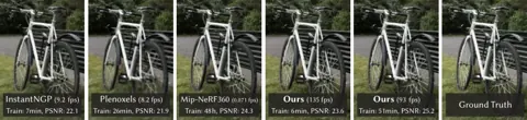
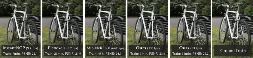
Fig. 13DGS 即時渲染品質與訓練時間,與 Mip-NeRF360、InstantNGP、Plenoxels 比較
出處:Kerbl et al., 2023,Fig. 1。授權:CC BY 4.0 (arXiv v1)。原始圖檔。修改:轉存為 WebP 格式。

Fig. 2方法總覽:由 SfM 稀疏點建立三維高斯,最佳化並自適應控制密度,再以分塊光柵化渲染
出處:Kerbl et al., 2023,Fig. 2。授權:CC BY 4.0 (arXiv v1)。原始圖檔。修改:轉存為 WebP 格式。
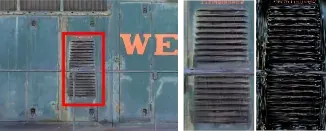
Fig. 3將最佳化後的三維高斯縮小 60% 以顯示其各向異性形狀
出處:Kerbl et al., 2023,Fig. 3。授權:CC BY 4.0 (arXiv v1)。原始圖檔。修改:轉存為 WebP 格式。
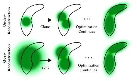
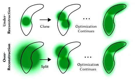
Fig. 4自適應密度控制:重建不足時複製高斯,過度重建時分裂高斯
出處:Kerbl et al., 2023,Fig. 4。授權:CC BY 4.0 (arXiv v1)。原始圖檔。修改:轉存為 WebP 格式。

作者報告的優勢與限制
優勢
- Real-time radiance-field rendering with high visual quality (abstract)
- On Mip-NeRF360, PSNR 27.21 at 30K iterations vs 27.69 reported for Mip-NeRF360, with 41 min vs 48 h training and 134 FPS vs 0.06 FPS (Table 1)
- At 7K iterations quality is comparable to InstantNGP and Plenoxels with similar training time (Sec. 7.2, Table 1)
限制
- Artifacts in poorly observed regions; elongated or 'splotchy' Gaussians; popping artifacts (Sec. 7.4)
- No regularization applied to the optimization (Sec. 7.4)
- Follow-up work states 3DGS fails to accurately represent surfaces because 3D Gaussians are multi-view inconsistent ((Huang et al., 2024a) abstract)
- Memory consumption is significantly higher than NeRF-based solutions: peak training memory can exceed 20 GB on large scenes and stored models reach hundreds of MB (Sec. 7.4, Table 1)
- Very large scenes such as urban datasets may need a reduced position learning rate (Sec. 7.4)
- Views with little overlap with training views show artifacts (Fig. 12)
營建工程相關證據
原論文未涉及營建;AEC 中 3DGS 與 LiDAR 的比較見(Yu et al., 2025)。
原文驗證環境:公開基準
報告的性能數據
以下是原文作者報告的性能數值(author-reported results),不是本研究重新量測的結果。每張圖只並列同一個比較組(comparison group,同一張表、同一組實驗設定)內的方法;不同比較組之間的數值不可直接比較,也不構成排名。
本方法共出現在 12 個比較組,合計 130 筆紀錄。以下列出本方法紀錄最多的 4 組,其餘 8 組列在最後,並連到性能比較頁。
Kerbl et al., 2023 · Table 1 本方法 36 筆
表格設定(擷取紀錄原文):Novel-view synthesis on held-out views (every 8th photo), average per dataset, with training time, rendering FPS and model memory; all on an A6000 GPU except Mip-NeRF360 (trained on a 4-GPU A100 node for 12 h, stated as 48 h single-GPU equivalent); dagger values copied from the Mip-NeRF360 paper (Kerbl et al., 2023, Table 1)
SSIM,Tanks&Temples · dataset average
只並列這張表在相同設定下報告的方法;以「本方法:」開頭者為本頁方法。失敗、未執行與未報告以標記呈現,不是 0。
按 Tab 進入圖表後,用上下方向鍵逐一瀏覽各類別,Esc 關閉提示框;也可開啟表格檢視閱讀全部數值。
這些是 Kerbl et al., 2023 在此表設定下報告的數值(author-reported results),只能在同一個比較組內對照,不代表方法在其他資料或設定下的表現。
資料來源作者報告值(Kerbl et al., 2023, Table 1)
| 方法(原文寫法) | 報告值 | 出處 |
|---|---|---|
| Plenoxels | 0.719 | (Kerbl et al., 2023, Table 1) |
| INGP-Base | 0.723 | (Kerbl et al., 2023, Table 1) |
| INGP-Big | 0.745 | (Kerbl et al., 2023, Table 1) |
| M-NeRF360 | 0.759 | (Kerbl et al., 2023, Table 1) |
| Ours-7K本方法原文提出 | 0.767 | (Kerbl et al., 2023, Table 1) |
| Ours-30K本方法原文提出 | 0.841 | (Kerbl et al., 2023, Table 1) |
Hong et al., 2024 · Table III 本方法 18 筆
表格設定(擷取紀錄原文):Ablation of map structure optimization: Case I = 3D-GS baseline; Case II = LiDAR-initialized Gaussians without visual structure optimization; Case III = Case II plus photometric position optimization; Case IV = full method with Gaussian pose refinement; SSIM and LPIPS rows of this table omitted here; Cases II and III are ablation variants (method_id null) (Hong et al., 2024, Table III)
PSNR [dB] (Interpolated),FAST-LIVO dataset · HKU_MB(outdoor)
只並列這張表在相同設定下報告的方法;以「本方法:」開頭者為本頁方法。失敗、未執行與未報告以標記呈現,不是 0。
按 Tab 進入圖表後,用上下方向鍵逐一瀏覽各類別,Esc 關閉提示框;也可開啟表格檢視閱讀全部數值。
這些是 Hong et al., 2024 在此表設定下報告的數值(author-reported results),只能在同一個比較組內對照,不代表方法在其他資料或設定下的表現。
資料來源作者報告值(Hong et al., 2024, Table III)
| 方法(原文寫法) | 報告值 | 出處 |
|---|---|---|
| Case I (3D-GS baseline)本方法 | 24.39 dB | (Hong et al., 2024, Table III) |
| Case II (LiDAR initialization only) | 24.341 dB | (Hong et al., 2024, Table III) |
| Case III (+ photometric position optimization) | 24.24 dB | (Hong et al., 2024, Table III) |
| Case IV (full method)原文提出 | 25.14 dB | (Hong et al., 2024, Table III) |
Huang et al., 2024a · Table 1 本方法 17 筆
表格設定(擷取紀錄原文):Chamfer distance per DTU scan (15 scans) and mean; meshes of 3DGS and 2DGS by TSDF fusion of rendered depth; unit not stated in the paper; images downsampled to 800 x 600; COLMAP sparse points for initialization (Huang et al., 2024a, Table 1)
Chamfer distance (CD),DTU · scan 24
只並列這張表在相同設定下報告的方法;以「本方法:」開頭者為本頁方法。失敗、未執行與未報告以標記呈現,不是 0。
按 Tab 進入圖表後,用上下方向鍵逐一瀏覽各類別,Esc 關閉提示框;也可開啟表格檢視閱讀全部數值。
這些是 Huang et al., 2024a 在此表設定下報告的數值(author-reported results),只能在同一個比較組內對照,不代表方法在其他資料或設定下的表現。
資料來源作者報告值(Huang et al., 2024a, Table 1)
| 方法(原文寫法) | 報告值 | 出處 |
|---|---|---|
| NeRF (Mildenhall et al., 2021) | 1.9 | (Huang et al., 2024a, Table 1) |
| VolSDF (Yariv et al., 2021) | 1.14 | (Huang et al., 2024a, Table 1) |
| NeuS (Wang et al., 2021) | 1 | (Huang et al., 2024a, Table 1) |
| 3DGS (Kerbl et al., 2023)本方法 | 2.14 | (Huang et al., 2024a, Table 1) |
| SuGaR (Guédon and Lepetit, 2023) | 1.47 | (Huang et al., 2024a, Table 1) |
| 2DGS-15k (Ours)原文提出 | 0.48 | (Huang et al., 2024a, Table 1) |
| 2DGS-30k (Ours)原文提出 | 0.48 | (Huang et al., 2024a, Table 1) |
Hong et al., 2024 · Table II 本方法 16 筆
資料集與序列not stated (real-world dataset) · not stated
表格設定(擷取紀錄原文):Novel-view synthesis on interpolated and extrapolated views on a real-world dataset (dataset and sequence not named for this table); asterisk methods were enhanced with dense LiDAR point clouds; cost time and FPS on the authors' desktop (Hong et al., 2024, Table II)
PSNR (Interpolate),not stated (real-world dataset) · not stated
只並列這張表在相同設定下報告的方法;以「本方法:」開頭者為本頁方法。失敗、未執行與未報告以標記呈現,不是 0。
按 Tab 進入圖表後,用上下方向鍵逐一瀏覽各類別,Esc 關閉提示框;也可開啟表格檢視閱讀全部數值。
這些是 Hong et al., 2024 在此表設定下報告的數值(author-reported results),只能在同一個比較組內對照,不代表方法在其他資料或設定下的表現。
資料來源作者報告值(Hong et al., 2024, Table II)
| 方法(原文寫法) | 報告值 | 出處 |
|---|---|---|
| Point-NeRF* [2] | 27.331 dB | (Hong et al., 2024, Table II) |
| DS-NeRF* [24] | 27.178 dB | (Hong et al., 2024, Table II) |
| 3D-GS* [1]本方法 | 31.9 dB | (Hong et al., 2024, Table II) |
| Plenoxel [18] | 26.744 dB | (Hong et al., 2024, Table II) |
| M-NeRF360 [16] | 28.446 dB | (Hong et al., 2024, Table II) |
| F2-NeRF [25] | 32.556 dB | (Hong et al., 2024, Table II) |
| 3D-GS [1]本方法 | 31.899 dB | (Hong et al., 2024, Table II) |
| Our method原文提出 | 32.787 dB | (Hong et al., 2024, Table II) |
其他比較組
來源
Kerbl et al., 2023
(2023)3D Gaussian Splatting for Real-Time Radiance Field RenderingACM Transactions on Graphics, 42(4), 1-14
DOI 10.1145/3592433arXiv 2308.04079程式碼
同儕審查已出版已讀全文近十年查證後修正
相關版本
- 預印本:arXiv:2308.04079 (posted after the TOG online date) https://arxiv.org/abs/2308.04079
程式碼:https://github.com/graphdeco-inria/gaussian-splatting(授權:Gaussian-Splatting License (custom Inria/MPII licence: research use, non-commercial only; commercial use prohibited without licensor consent; LICENSE.md read))。有公開程式碼不等於已被重現,也不代表目前版本與論文版本相同。